When a query requires data from more than one table, the accessed tables are joined two at a time. The WHERE clause, or filter, in the query determines the criteria for selecting rows from the tables.
The method and order in which the optimizer chooses to join the tables is the join plan. Different join methods have join tables differently and have specific advantages and disadvantages, as described in the following sections.
If a generalized-key (GK) index has been created to contain the result of a join on STATIC tables, the database server uses the GK index instead of joining the table columns again. For more information on the requirements for this kind of index, refer to Creating Specialized Indexes.
In a nested-loop join, the optimizer selects one of the joined tables as the outer table and the other table as the inner table. The database server scans the outer table row by row. For each row in the outer table, the database server scans the inner table to find a matching row.
A nested-loop join might be efficient in both of the following conditions are met:
A nested-loop join is inefficient if the outer table is large or the number of required rows in the outer table cannot be reduced by the filter or if the inner table does not have an index on the join column.
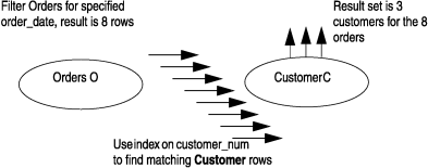
Figure 30 shows the plan for the following query:
SELECT * FROM customer C, orders O
WHERE o.order_date > "01/01/97" AND c.customer_num =
o.customer_num.
Nested-loop joins between large tables should be avoided whenever possible. In the example shown in Figure 30, in which the outer table is unrealistically small, a nested-loop query performs well. However, if the outer table contained sixty thousand rows instead of eight filtered rows, a nested-loop join might not be appropriate.
A hash join method of joining two tables consists of two parts: the build phase and the probe phase. The optimizer uses statistical information created by the UPDATE STATISTICS statement and other cost estimates to determine which of the two tables is smaller or will produce a smaller hash table, then it builds the hash table on the join key of that table. The best performance results when the hash table can be built entirely in shared memory.
The probe phase begins after the hash table is built. The hash buckets, formally called partitions, can easily be processed in parallel by several CPU virtual processors and across several coservers for even greater efficiency. The database server reads rows in the probe table, applies the hash function to the join keys in the row and looks up -- or probes -- the join key values in the matching partition of the hash table. Only the hash bucket that contains rows with the same key-value hash result need be probed to match the join key.
Small hash tables can fit in the virtual portion of the database server shared memory. If the database server runs out of memory, hash tables are overflow to the dbspaces specified by the DBSPACETEMP configuration parameter or environment variable.
Hash joins are well suited to parallel processing because they can be executed on all CPU virtual processors of all coservers that host fragments of the joined tables. Hash joins and other uses of hash functions are effective in balancing query processing or data distribution only if the hashed column does not contain many duplicates. For hash joins, if the join key column contains many duplicates, one hash partition will contain many more rows than other partitions. This condition creates one kind of data skew. Performance suffers because the other coservers must wait for the coserver that is processing the largest hash table.
The following example query runs against a database with a modified fact-dimension schema that does not join each dimension table directly to the fact table in the schema. The join plan for this query might be the series of hash joins shown in:
SELECT *
FROM sales s, location l, customer c, agent a,
WHERE s.state_id = l.state_id
   AND l.region_id = c.region_id
   AND c.agent  = a.agent
   ...
Figure 31 shows a simple left-deep hash-join plan. Left-deep indicates that the hash joins are on the left side of the query plan diagram as data moves from bottom to top.
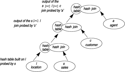
Push-down hash joins, which are described in the following section, use right-deep join plans.
Push-down hash joins are used only for tables in a star or snowflake schema. These schemas, often used for data warehouses and data marts, consist of one or two very large fact tables joined by foreign keys to several very small dimension tables. For information about star and snowflake schemas, refer to the IBM Informix: Database Design and Implementation Guide.
The primary purpose of a push-down hash join is to reduce the size of the initial probe table, usually a fact table. In a push-down hash-join plan, all of the hash tables are built before any hash joins occur. The database server pushes down one or more of the join keys to filter the fact table at the same time as it builds hash tables on the dimension tables. This dynamic filter on the fact table reduces the number of rows used in the probe phase of the actual hash joins. A more descriptive name for push-down hash joins might be push-down filters.
The database server can choose a push-down hash join for star or snowflake schema queries in the following circumstances:
For information about adjusting the optimizer decision to choose a push-down hash join, see Prevent or Encourage Push-Down Hash Joins.
The plan for the following query might use a push-down hash join to filter the rows in the orders table before these rows are sent to the next hash join operator. The orders table does not probe the customer hash table until it has been filtered by the location_id keys pushed down during the build of the location hash table.
SELECT t.quarter, o.sum(quantity)
FROM orders o, customer c, location l, time t
WHERE    o.cust_id = c.cust_id
       AND o.location_id = l.location_id
       AND o.time_id = t.time_id
        AND t.quarter between 1 and 20
       AND c.cust_type <= 3
       AND  l.region_id = 4
GROUP BY t.quarter;
Push-down hash-join plans use right-deep plans, in which the hash joins appear on the right side of the plan diagram. Figure 32 illustrates push-down hash join plan for the previous query.
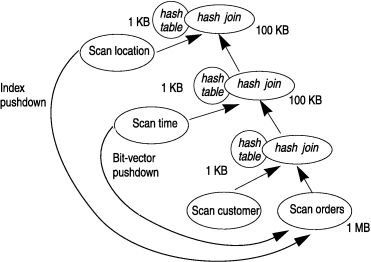
Hash tables are built first on the location and time tables, then on the customer table. The hash table created from the location table contains only the filtered rows of the table that meet the filter requirements l.region_id = '4'. For these filtered rows, the location_id keys are pushed down in the query processing plan and applied as filters to the orders fact table. Keys are also pushed down from time hash table build to filter the orders fact table. Filtering the rows of the orders table to select only rows with states included in region four and times that correspond to quarters one through twenty reduces the size of the probe table in all of the subsequent hash joins.
In a zigzag hash join, the optimizer examines distribution statistics for the joined tables and decides whether a left-deep or right-deep hash join would be more efficient for each join. As a result, a query-plan diagram would show the some hash joins with the probe table on the left, and some hash joins with the probe table on the right.
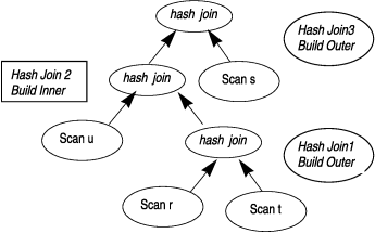
Figure 33 shows a schematic diagram of the hash-join plan that is described by the following SET EXPLAIN output.
QUERY:
------
select * from r, t, u, s where r.a = s.a and r.b = t.b and r.c =
u.c
Estimated Cost: 3647
Estimated # of Rows Returned: 9375
1) sales.r: SEQUENTIAL SCAN (Parallel, fragments: ALL)
2) sales.t: SEQUENTIAL SCAN (Parallel, fragments: ALL)
DYNAMIC HASH JOIN (Build Outer)
  Dynamic Hash Filters: sales.r.b = sales.t.b

3) sales.u: SEQUENTIAL SCAN (Parallel, fragments: ALL)
DYNAMIC HASH JOIN (Build Inner)
  Dynamic Hash Filters: sales.r.c = sales.u.c

4) sales.s: SEQUENTIAL SCAN (Parallel, fragments: ALL)
DYNAMIC HASH JOIN (Build Outer)
  Dynamic Hash Filters: sales.r.a = sales.s.a

# of Secondary Threads = 14
XMP Query Plan
  oper   segid  brid width misc info
  -----------------------------------------
  scan     4     0    2        r
  scan     5     0    2        t
  hjoin    3     0    2
  scan     6     0    2        u
  hjoin    2     0    2
  scan     7     0    2        s
  hjoin    1     0    2
Implicit PDQ Priority

set environment IMPLICIT_PDQ       10 %
Ideal Implicit PDQ Priority      1350 %
Requested Implicit PDQ Priority   135 %
Granted Implicit PDQ Priority      80 %
Ideal Query Memory        216676 KB/coserver
Requested Query Memory    21668 KB/coserver
Granted Query Memory      12800 KB/coserver
Home | [ Top of Page | Previous Page | Next Page | Contents | Index ]