Statistics
Basic statistics
- Average/Mean (μ): An average is most commonly an arithmetic mean of a set of values, calculated as the sum of a set of values, divided by the count of values: μ = (x1 + x2 + ... + xN)/N. For example, to calculate the average of the set of values (10, 3, 3, 1, 99), sum the values (116), and divide by the count, 5 (μ=23.2).
- Median: A median is the middle value of a sorted set of values. For example, to calculate the median of the set of values (10, 3, 3, 1, 99), sort the values (1, 3, 3, 10, 99), and take the midpoint value (3). If the count of values is even, then the median is the average of the middle two values.
- Mode: A mode is the value that occurs most frequently. For example, to calculate the mode of the set of values (10, 3, 3, 1, 99), find the value that occurs the most times (3). If multiple values share this property, then the set is multi-modal.
- Standard Deviation (σ): A standard deviation is a measure of how far a set of values are spread out relative to the mean, with a standard deviation of zero meaning all values are equal, and more generally, the smaller the standard deviation, the more the values are closer to the mean. If the set of values is the entire population of values, then the population standard deviation is calculated as the square root of the average of the squared differences from the mean: σ = √( ( (x1 - μ)2 + (x2 - μ)2 + ... + (xN - μ)2 ) / N ). If the set of values is a sample from the entire population, then the sample standard deviation uses the division (N - 1) instead of N.
- Confidence Interval: A confidence interval describes the range of values in which the true mean has a high likelihood of falling (usually 95%), assuming that the original random variable is normally distributed, and the samples are independent. If two confidence intervals do not overlap, then it can be concluded that there is a difference at the specified level of confidence in performance between two sets of tests.
- Relative change: The ratio of the difference of a new quantity (B) minus an old quantity (A) to the old quantity: (B-A)/A. Multiply by 100 to get the percent change. If A is a "reference value" (e.g. theoretical, expected, optimal, starting, etc.), then relative/percent change is relative/percent difference.
Small sample sizes (N) and large variability (σ) decrease the likelihood of correct interpretations of test results.
Here is R code that shows each of these calculations (the R project is covered under the Major Tools chapter):
> values=c(10, 3, 3, 1, 99)
> mean(values)
[1] 23.2
> median(values)
[1] 3
> summary(values) # A quick way to do the above
   Min. 1st Qu.  Median    Mean 3rd Qu.    Max.
    1.0     3.0     3.0    23.2    10.0    99.0
> mode = function(x) { ux = unique(x); ux[which.max(tabulate(match(x, ux)))] }
> mode(values)
[1] 3
> sd(values) # Sample Standard Deviation
[1] 42.51118
> error = qt(0.975,df=length(values)-1)*(sd(values)/sqrt(length(values)))
> ci = c(mean(values) - error, mean(values) + error)
> ci # Confidence Interval at 95%
[1] -29.5846  75.9846
Amdahl's Law
Amdahl's Law states that the maximum expected improvement to a system when adding more parallelism (e.g. more CPUs of the same speed) is limited by the time needed for the serialized portions of work. The general formula is not practically calculable for common workloads because they usually include independent units of work; however, the result of Amdahl's Law for common workloads is that there are fundamental limits of parallelization for system improvement as a function of serialized execution times.
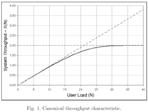
In general, because no current computer system avoids serialization completely, Amdahl's Law shows that, all other things equal, the throughput curve of a computer system will approach an asymptote (which is limited by the bottlenecks of the system) as number of concurrent users increases:
Relatedly, response times follow a hockey stick pattern once saturation occurs:
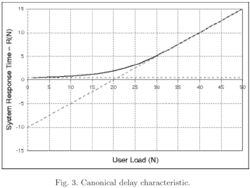
Fig. 3 shows the canonical system response time characteristic R (the dark curve). This shape is often referred to as the response hockey stick. It is the kind of curve that would be generated by taking time-averaged delay measurements in steady state at successive client loads. The dashed lines in Fig. 3 also represent bounds on the response time characteristic. The horizontal dashed line is the floor of the achievable response time Rmin. It represents the shortest possible time for a request to get though the system in the absence of any contention. The sloping dashed line shows the worst case response time once saturation has set in.
Queuing Theory
Queuing theory is a branch of mathematics that may help model, analyze, and predict the behavior of queues when requests (e.g. HTTP requests) flow through a set of servers (e.g. application threads) or a network of queues. The models are approximations with various assumptions that may or may not be applicable in real world situations. There are a few key things to remember:
- A server is the thing that actually processes a request (e.g. an application thread).
- A queue is a buffer in front of the servers that holds requests until a server is ready to process them (e.g. a socket backlog, or a thread waiting for a connection from a pool).
- The arrival rate (λ) is the rate at which requests enter a queue. It is often assumed to have the characteristics of a random/stochastic/Markovian distribution such as the Poisson distribution.
- The service time (µ) is the average response time of servers at a queue. Similar to the arrival rate, it is often assumed to have the characteristics of a Markovian distribution such as the Exponential distribution.
- Queues are described using Kendall's
notation: A/S/c
- A is the distribution of arrivals, which is normally M for Markovian (e.g. Poisson),
- S is the distribution of service times, which is normally M for Markovian (e.g. Expontential),
- c is the number of concurrent servers (e.g. threads).
- Therefore, the most common type of a queue we will deal with is an M/M/c queue.
For example, we will model a typical three tier architecture with a web server (e.g. IHS), application server (e.g. WAS), and a database:
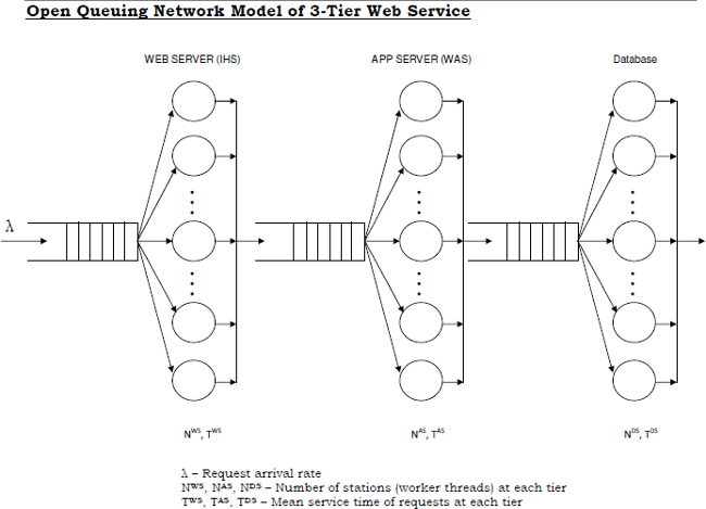
This is a queuing network of three multi-server queues in series. Steady state analysis can be done by analyzing each tier independently as a multi-server M/M/c queue. This is so because it was proved that in a network where multi-server queues are arranged in series, the steady state departure processes of each queue are the same as the arrival process of the next queue. That is, if the arrival process in the first multi-server queue is Poisson with parameter λ then the steady state departure process of the same queue will also be Poisson with rate λ, which means the steady state arrival and departure processes of the 2nd multi-server queue will also be Poisson with rate λ. This in turn means that the steady state arrival and departure processes of the 3rd multi-server queue will also be Poisson with rate λ.
Assumptions:
- The arrival process is Poisson with rate λ. That is, the
inter-arrival time T1 between arrivals of two successive requests
(customers) is exponentially distributed with parameter λ. This
means:

- The service rate of each server is exponentially distributed with
parameter µ, that is the distribution of the service time is:

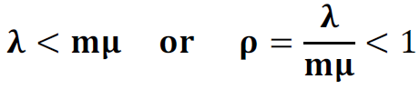
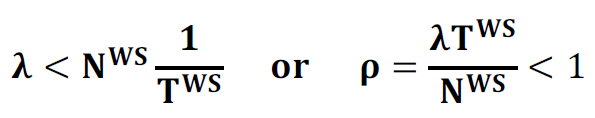
1. Stability Condition: The arrival rate has to be less than the service rate of m servers together. That is:
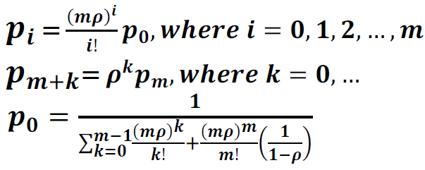
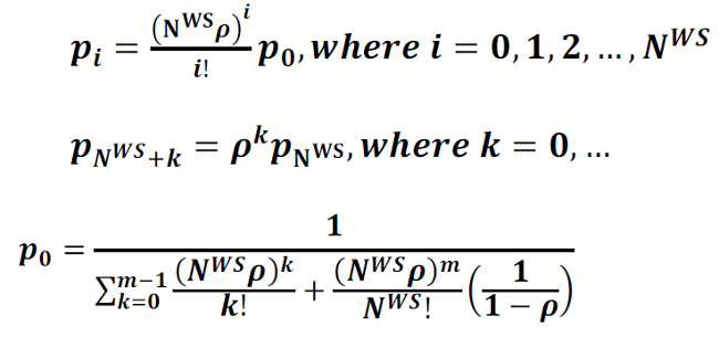
2. State Occupancy Probability:
pi = Probability that there are i customers (requests) in the system (at service)
pm+k = Probability that there are m+k customers (requests) in the system (m at service and k waiting in the queue)
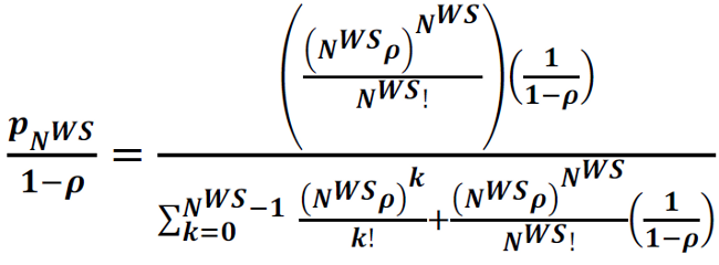
3. Probability that a Customer (Request) has to Wait:
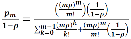
4. Expected number of Busy Servers:
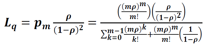
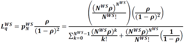
5. Expected number of Waiting Requests:
6. Expected Waiting Time in the Queue:
7. Expected Waiting Time in the Queue:
8. Expected Waiting Time in the System:
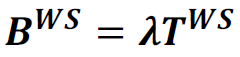
To obtain performance measures of the Web Server, Application Server and Database Server, we replace m in the above given formulae by NWS, NAS and NDS, respectively and replace µ by 1/TWS, 1/TAS and 1/TDS, respectively. As an example, the performance measures for the Web Server are given below. The performance measures for App Server and the DB Server can be obtained in the same way.
1W. Stability Condition for Web Server Queue:
2W. Web Server State Occupancy Probability:
pi = Probability that there are i customers (requests) in the system (at service)
pNws+k= Probability that there are NWS+k customers (requests) in the system (NWS at service and k waiting in the queue)
3W. Probability that a Customer (Request) has to Wait at the Web Server:
4W. Expected number of Busy Web Servers:
5W. Expected number of Requests Waiting at the Web Server Queue:
6W. Expected Waiting Time in the Web Server Queue:
7W. Expected number of Requests in the Web Server:
8W. Expected Waiting Time in the Web Server:
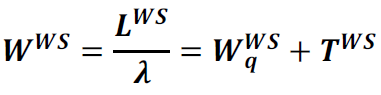
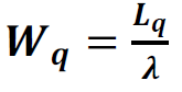
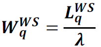
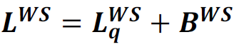
Little's Law
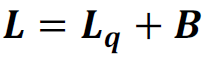
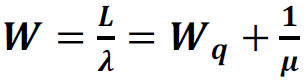
Little's Law states that the long-term average number of requests in a stable system (L) is equal to the long-term average effective arrival rate, λ, multiplied by the (Palm‑)average time a customer spends in the system, W; or expressed algebraically: L = λW.
Practical Queuing Theory
The key takeaways from above are that queues are largely a function of three variables: arrival rate, number of threads, and service time which may be visualized with the following key performance indicators (KPIs):
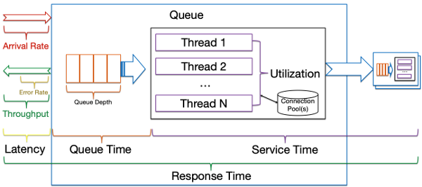
There are seven key things that ideally should be monitored at as many layers as possible, both for diagnosing performance problems and planning for scalability:
- Service Time: the average time it takes to complete a request by a server thread. Think of a cashier at a supermarket and the average time it takes a cashier to check out a customer.
- Utilization: the total number of available server threads and the average percentage used. Think of the number of cashiers at a supermarket and the average percentage actively processing a customer.
- Arrival Rate: the rate at which work arrives at the queue. Think of the rate at which customers arrive at a supermarket checkout line.
- Response Time: the average time it takes to wait in the queue plus the service time. Think of the average time it takes a customer to stand in line at a checkout line plus the average time it takes a cashier to check out a customer.
- Queue Depth: the average size of the waiting queue. Think of the average number of customers at a supermarket waiting in a queue of a checkout line.
- Error Rate: the rate of errors processing requests. Think of the rate at which customers at a supermarket fail to complete a check out and leave the store (on the internet, they might immediately come back by refreshing).
- Latency: The time spent in transit to the queue.
The above six statistics will be called Key Queue Statistics (and OS CPU, memory, disk, and network can be included as well). For this infrastructure, an ideal interval at which to capture these statistics seems to be every 10 seconds (this may need to be increased for certain components to reduce the performance impact).
Throughput is simply the number of completed requests for some unit of time. Throughput may drop if service time increases, the total number of available server threads decreases, and/or the arrival rate decreases (when server thread utilization is less than 100%).
For performance analysis, a computer infrastructure may be thought of as a network of queues (there's no supermarket analogy because you don't check out of one line and queue into another check out line). The IHS queue feeds the WAS queue which feeds the DB2 queue and so on. Roughly speaking, the throughput of an upstream queue is usually proportional to the arrival rate of the downstream queue.
Each one of these queues may be broken down into sub-queues all the way down to each CPU or disk being a queue; however, in general, this isn't needed and only the overall products can be considered. From the end-user point of view, there's just a single queue: they make an HTTP request and get a response; however, to find bottlenecks and scale, we need to break down this one big queue into a queuing network.
It is common for throughput tests to drive enough load to bring a node to CPU saturation. Strictly speaking, if the CPU run queue is consistently greater than the number of CPU threads, since CPUs are not like a classical FIFO queue but instead context switch threads in and out, then throughput may drop as service time increases due to these context switches, reduced memory cache hits, etc. In general, the relative drop tends to be small; however, an ideal throughput test would saturate the CPUs without creating CPU run queues longer than the number of CPU threads.
Response Times and Throughput
Response times impact throughput directly but they may also impact throughput indirectly if arrivals are not independent (e.g. per-user requests are temporally dependent) as is often the case for human-based workloads such as websites.
As a demonstration, imagine that two concurrent users arrive at time 00:00:00 (User1 & User2) and two concurrent users arrive at time 00:00:01 (User3 & User4). Suppose that each user will make three total requests denoted (1), (2) and (3). Suppose that (2) is temporally dependent on (1) in the sense that (2) will only be submitted after (1) completes. Suppose that (3) is temporally dependent on (2) in the sense that (3) will only be submitted after (2) completes. For simplicity, suppose that the users have zero think time (so they submit subsequent requests immediately after a response). Then suppose two scenarios: average response time = 1 second (columns 2 and 3) and average response time = 2 seconds (columns 4 and 5):
Request    Arrived (μ=1s)  Completed (μ=1s)    Arrived (μ=2s)  Completed (μ=2s)
User1(1)   00:00:00        00:00:01            00:00:00        00:00:02
User1(2)   00:00:01        00:00:02            00:00:02        00:00:04
User1(3)   00:00:02        00:00:03            00:00:04        00:00:06
User2(1)   00:00:00        00:00:01            00:00:00        00:00:02
User2(2)   00:00:01        00:00:02            00:00:02        00:00:04
User2(3)   00:00:02        00:00:03            00:00:04        00:00:06
User3(1)   00:00:01        00:00:02            00:00:01        00:00:03
User3(2)   00:00:02        00:00:03            00:00:03        00:00:05
User3(3)   00:00:03        00:00:04            00:00:05        00:00:07
User4(1)   00:00:01        00:00:02            00:00:01        00:00:03
User4(2)   00:00:02        00:00:03            00:00:03        00:00:05
User4(3)   00:00:03        00:00:04            00:00:05        00:00:07
The throughput will be as follows:
Time                       Throughput/s (μ=1s)                 Throughput/s (μ=2s)
00:00:01                   2                                   0
00:00:02                   4                                   2
00:00:03                   4                                   2
[...]
Note that in the above example, we are assuming that the thread pool is not saturated. If the thread pool is saturated then there will be queuing and throughput will be bottlenecked further.
Of course, ceteris paribus, total throughput is the same over the entire time period (if we summed over all seconds through 00:00:07); however, peak throughput for any particular second will be higher for the lower response time (4 vs. 2). In addition, ceteris paribus often will not hold true because user behavior tends to change based on increased response times (e.g. fewer requests due to frustration [in which case total throughput may drop]; or, more retry requests due to frustration [in which case error throughput may increase]).
Tuning Timeouts
- For On-Line Transaction Processing (OLTP) systems, human perception may be assumed to take at least 400ms; therefore, an ideal timeout for such systems is about 500ms.
- One common approach to setting timeouts based on historical data is to calculate the 99th percentile response time from historical data from healthy days. An alternative is to use the maximum response time plus 20%. Note that both of these approaches often capture problematic responses which should not be considered healthy; instead, consider plotting the distribution of response times and take into account expectations of the system and business requirements.
- Timeouts should be set with all stakeholders involved as there may be known times (e.g. once per month or per year) that are expected to be high.
- If systems allow it (e.g. IBM HTTP Server with websphere-serveriotimeout), consider setting an aggressive global timeout and then override with longer timeouts for particular components that are known to take longer (e.g. report generation).
- In general, timeouts should follow a "funnel model" with the largest timeouts nearer to the user (e.g. web server) and lower timeouts in the application/database/etc.
Determining Bottlenecks
There are three key variables in evaluating bottlenecks at each layer of a queuing network:
- Arrival rate
- Concurrency
- Response time
These are also indirectly affected by many variables. For example, CPU saturation will impact response times and, with sufficient queuing, concurrency as a thread pool saturates; TCP retransmits or network saturation will impact arrival rate and response times, etc.
Common tools to investigate arrival rates and response times include access logs and averaged monitoring statistics. Common tools to investigate concurrency and excessive response times are averaged monitoring statistics and thread dumps.